
The early days of wind- and PV-power were rough: the engineers fought against oil-leaks in the pitch-mechanism of wind-power-systems and PV-inverters lived up to their German name “Wechselrichter” (wechsel = change) in an unfortunate way, as they had to be replaced very often due to defects. But since the early 1990s lot of things have changed: the pitch-mechanism moved from a hydraulic- to an servo-electric-adjustment and PV-inverters got much more reliable. So both renewable energy-sources faced different challanges: in 2025 the total renewable energy was around 278 TWh, which is around 57% of the total electrical power of Germany. And as you know: with great power comes great responsibility.
So in 2012 the Federal Government of Germany published the SysTabV, the “Verordnung zur Gewährleistung der technischen Sicherheit und Systemstabilität des Elektrizitätsversorgungsnetzes (Systemstabilitätsverordnung – SysStabV)” which translates to “Ordinance on Ensuring the Technical Safety and System Stability of the Electricity Supply Network”. This very long law is better known as the 50.2Hz-problem: when lot of energy is available in the public grid, the frequency rises and vice versa. The old PV-inverters disconnected from the grid when the frequeny was above the 50.2Hz, resulting in an uncontrolled energy-drop that could (would) cause grid-instabilities. So inverters had to be upgraded to either reduce the fed-in power or mitigate the turn-off above a frequency of 50.2 Hz in a different way.
So what is the main-idea of this blog-post? I do not want to give a full lecture about inverters and its control, but give a brief overview and a practical example of a grid-supporting vector-controlled grid-tied inverter. To show the effect I will use the PLECS RT-Box real-time simulation-system to simulate an artificial grid and a TI C2000 microcontroller that contains the field-oriented control-loop.
Main components of an inverter
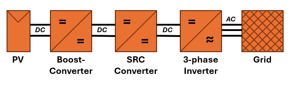
First we need a brief overview of what components are inside an inverter. The following picture will show the main-components of a PV-inverter but besides some minor details an inverter for wind-power will be very similar. The widely known device “inverter” contains different subsystems. On the left side we have the PV-modules (or the wind-generator) that generates a DC-voltage. As the PV-power fluctuates with the amount of radiation of the sun, a boost-converter is placed between the PV-DC-source and the subsequent devices. This boost-converter does nothing more than increase the input-voltage to a voltage with a gain-factor between 1.0 and 2.0. Higher gain-values are not feasible with the basic approach, but there are more complex converter-types we won’t discuss in this blog-post. Anyway, gain-factors between 1 and 2 are more than enough as we have a so called series-resonant-converter (SRC) connected to the boost-converter that allows two things: a galvanic isolation between source and sink and a fixed voltage-ratio that can be set by a high-frequency transformer. Finally the part of interest – our inverter – is connected to this SRC that converts the DC-voltage into a grid-compatible AC-voltage and AC-current:
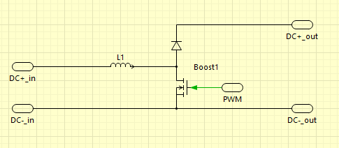
For the mentioned real-time-simulation the boost-converter uses only an inductor, a diode and a semiconductor-switch, like a MOSFET:
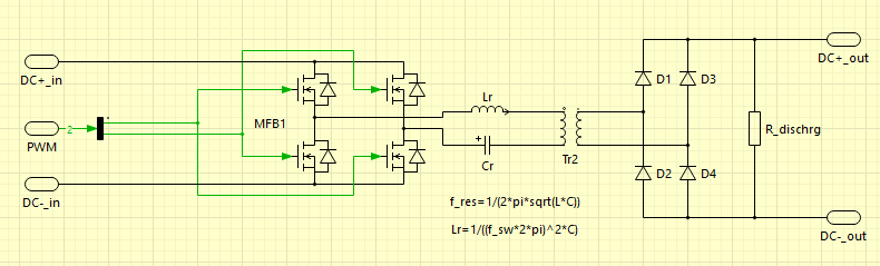
The series-resonant-converter looks like a single-phase inverter. It switches with a 50% duty-cycle and charges/discharges an inductor/capacitor-pair that is put in series with each other. As the charging/discharging is creating a high-frequent sine-wave, we can use a small high-frequency transformer to galvanically isolate the primary and secondary part of the circuit. On the secondary side we can use a simple full-bridge-rectifier to convert the sine-wave-voltage back to a DC-voltage:
Finally, the 3-phase inverter looks much easier compared to this SRC, as only six MOSFETs are used:
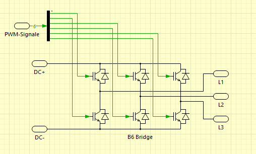
That’s it. Okay, I did not show the LCL-filter and the grid-relay, but these are the most important parts of the circuit. The whole magic lies wihtin the control-algorithms.
Realtime-simulation using PLECS RT Box
A couple of years ago I bought a PLECS RT Box, a realtime-simulation tool. It contains an FPGA that can be programmed using a model-based system. This RT Box can be connected to real-world-signals using a couple of connectors that contain analog- and digital signals. The next picture shows this system connected to a break-out-board for the TI C2000 LaunchPad-controller:
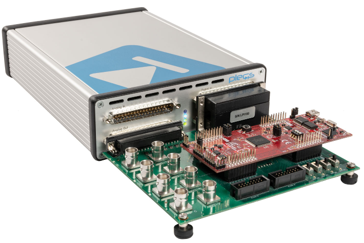
Within the RT Box I’ve implemented the individual parts shown above: the PV-plant, the boost-converter, the SRC-converter, the B6-3-phase-inverter and the LC-filter. The grid is realized using simple controllable voltage-sources. The whole structure looks like this:
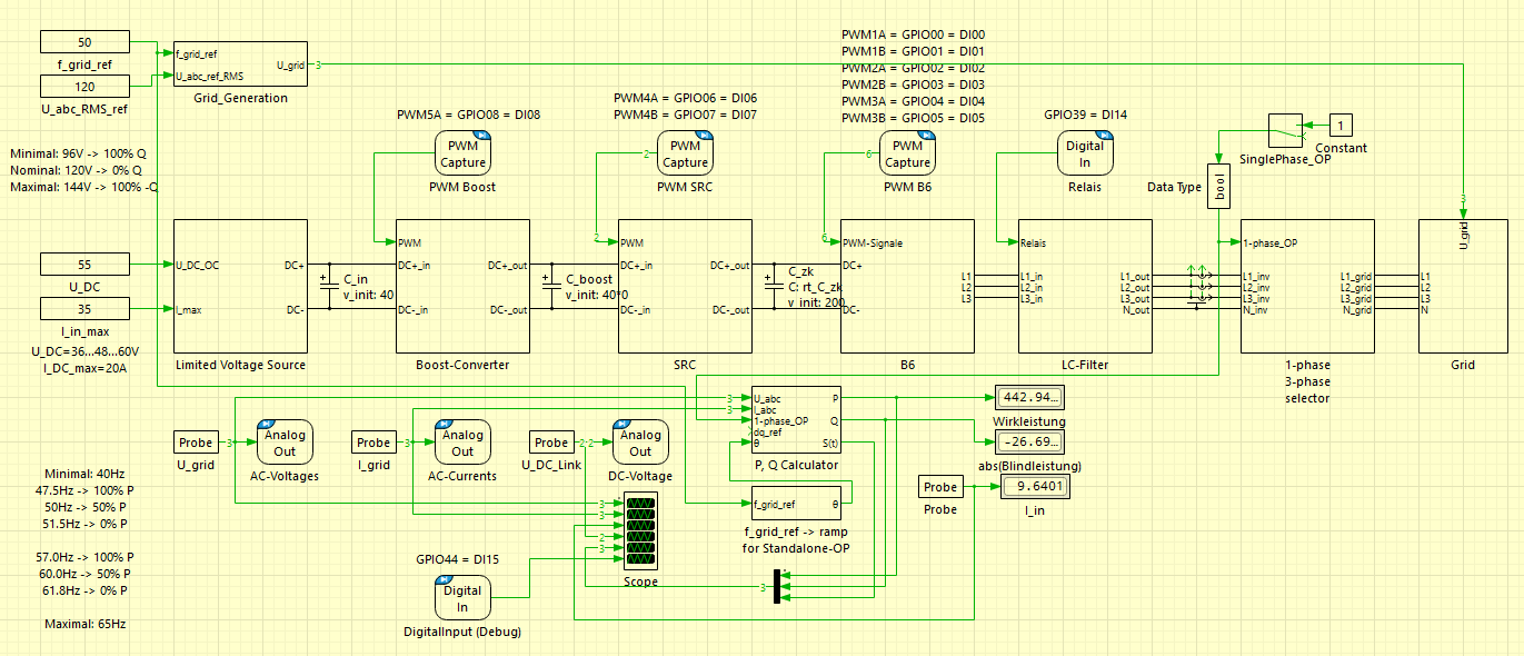
The RT Box uses PWM-capture-blocks to read the PWM-signals of the C2000 to control the simulated switches. Analog outputs allow the output of simulated voltages and currents to the C2000 microcontroller. A simple digital input is used to control the grid-relay. As this realtime-simulation-tool is connected via ethernet, the scope shown in the above picture displays the internal signals of the RT Box in realtime. So we can view the grid-voltages and -currents as well as other signals like the power on the computer-screen directly.
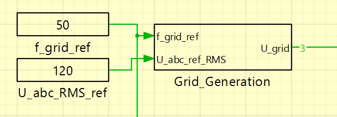
In the model I’m able to set the grid-frequency and the grid-voltages on the fly during the simulation. So I can emulate a over- or under-frequent grid or a voltage-drop or -rise using only two input-variables:
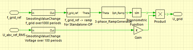
To mitigate a sudden change in the frequency or the voltage, I made use of a simple low-pass-filter. This filtered signal is then fed into an integrator that creates three common saw-tooth-signals with each 120° phase-shift with values between 0 and 2*Pi which can be used as a reference for the desired grid-currents:
Vector-controller for grid-tied inverters
As I said, I do not want to go into every detail of grid-tied inverters, but we need to talk about some very important parts. So here is the main-schematic of the main-system within the TI C2000 F28379D controller – click on the picture to see a larger version:
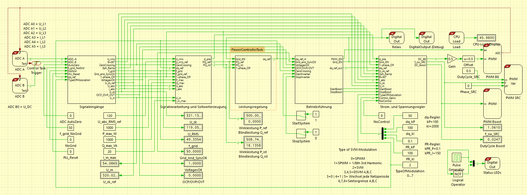
OK, you are still with me? Good… thought I lost you while looking at this mess 🙂 If we remove the hundrets of little connection-lines, the top-schematic can be reduced to five sub-blocks: the signal-inputs, the generation of the reference values, the power-controller, the operational management and the current-controller that creates the dutycycles for the PWM:

The signal-input-block contains one of the most-important blocks next to the current-controller: the so called phase-locked-loop (PLL). This PLL is responsible for the synchronisation of the controller to the grid. For this all three grid-voltages are taken into account to feed a so called phase-detector, a loop-filter and a so called voltage-controlled oscillator (VCO). The phase-detector compares the grid-voltages and feedback-signal phases and outputs an error signal proportional to their difference. The loop-filter smoothes this error signal by removing high-frequency noises and creates a steady control voltage. Finally this control-voltage is fed into the VCO that creates either a sawtooth-signal or real sinewave-signals that matches the frequency of the grid and acts as the reference signals of the whole inveter-control.
As the grid-voltages may contain disturbances, its crucial to have a resilient grid-synchronization even on high noises. So I decided to make use of the so called second-order generalized-integrator (SOGI) that I’ve used in the field-oriented control for my BLDC motor shown a couple of months ago on this blog. The full name is “Dual-Second-Order-Generalized-Integrator Quadrature Signal Generator with Frequency Locked Loop with Gain-Normilazation”…. pffffff. What a name. In short: next to the phase-locked loop it uses another feedback for the frequency to allow faster synchronization:
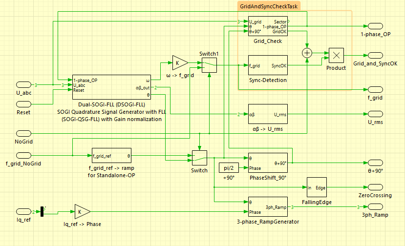
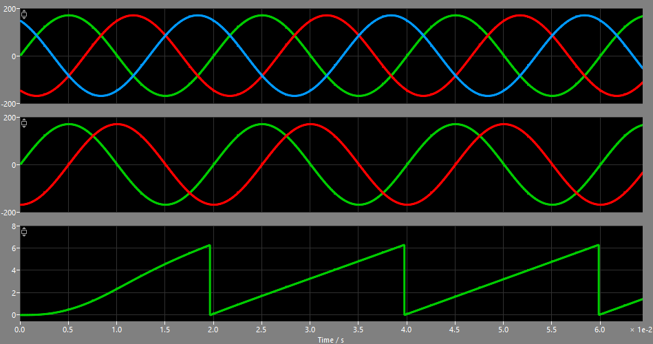
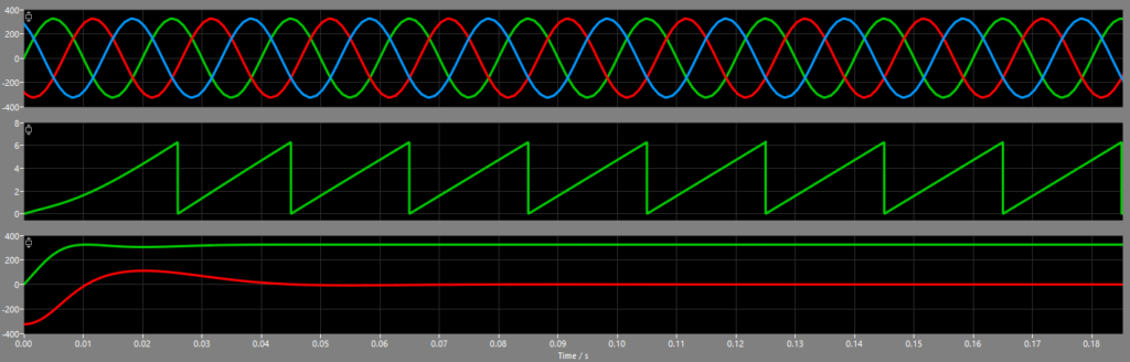
If you want more information, I suggest chapter 8 “Grid Synchronization in Three-Phase Power Converters” of Remus Teodorescu’s book “Grid Converters for Photovoltaic and Wind Power Systems” which shows all details with very good in-depth explanations. In the next graph you can see that the PLL only takes around 10ms to synchronize to the grid (beginning of the sawtooth is non-linear) and outputs a stable saw-tooth-signal after 20ms:
Now that we have a rough idea of what’s going in the first block of the control-system, lets jump to the last block, the current controller. Here most converters implement the so called FOC, the field-oriented control, or simply “vector control”. Let me demonstrate you what’s happening inside the vector control with a very professional picture:
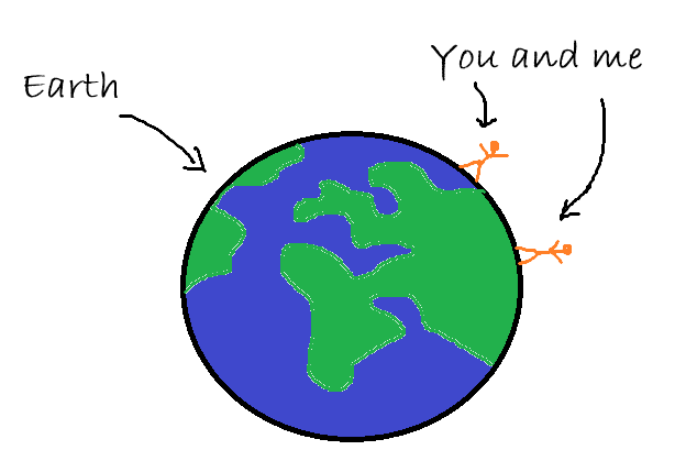
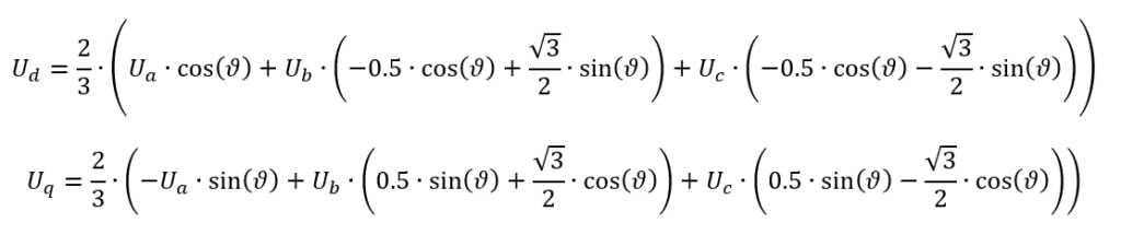
So, we are sitting on the surface of the earth which is rotating with a speed of around 1.000 km/h in Europe/Germany – but we still don’t get dizzy all time. Why? Because we are rotating with the surface of the earth and all reference points with us. But if you are looking up in the night, you realize the rotation when looking at the stars. And the same principle can be used for the grid – or better the rotor of a motor connected to the grid. A motor has a stator that is connected to the three phases of the grid and a rotor inside of the motor. The stator is not rotating, while the rotor does. So when you are looking from the stator to the rotor, the rotor rotates, but if you are sitting on the rotor, the rotors stands still and the surrounding stator is moving. Earth-Stars, Rotor-Stator… got it? So the main-idea of a field-oriented control is to look to the grid-currents while sitting on the rotor. So all voltages and currents have to be converted from the stator-reference-frame (SRF) to the rotor-reference-frame (RRF) which can be done with a combination of sine and cosine as well as the angle theta that acts as a control-angle for the rotation resulting in two equations for d- and q-part:
The next picture shows the three line-voltages L1, L2 and L3 of the grid in the top. The second signal is the sawtooth-signal (theta) of the PLL that locks to the three voltages of the grid. The third signal is the output of the SRF-to-RRF-conversion that displays only two components: d and q. “d” contains the combined amplitude of all three voltages, while “q” is the signal 90° to this voltage which is 0V when we are in sync to the grid.
Converting the voltages from SRF to RRF is one thing, but more useful is the conversion of the currents into the RRF. Here the q-current is responsible for the torque of the motor while the d-current is responsible for the field-control. Reducing the field-strength (hence field-weakening) is used to reach higher RPMs while reducing the impact of the permanent magnets. But we do not want to look at motors, but on the grid-application: in grid-applications the d-current is responsible for the active power fed into or pulled from the grid, while the q-part is related to the reactive power directly. This relationship is very important for the grid-supporting features lateron.
But first let’s have a look at the general idea of a field-oriented control. The following picture is from my blog-post about the FOC for the BLDC motor and shows the most important parts:
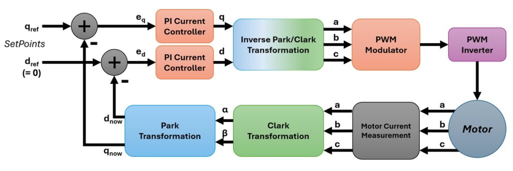
So we have a d/q-reference-current at the input that is compared to the actual d/q-currents from the motor after the Clark-Park-transformation. Then a simple PI-controller controls these two currents I_d and I_q. Using such a simple controller is only possible as we are dealing with DC-like-values as we are “sitting” on the rotor when using the rotor-reference-frame (RRF). So this PI-controller may have a small gain which makes the whole control-loop much easier to get stable compared to a controller that has to deal with time-variant sinewave-signals that changes with 50 Hz. To build the bridge to the grid-tied inverter simply replace the shown motor with the grid and you are done. The grid is “rotating” with 50 Hz and the whole control-loop can be used as if we would control a motor with very low impedance. And now you may realize: a motor-inverter, a PV-inverter and a wind-inverter are basically the same technology, only with different input-stages and minor changes regarding maximum-power-point-tracking or pitch-control for the rotor-blades.
Now only three blocks of the initial block-diagram are left: generation of the reference values, the power-controller and the operational management. The latter is only a state-machine-like block that takes care of the state of all safety-features, the check for under- and overvoltage and -current as well as the timed turn-on and -off of the individual components like the grid-relay. The generation of the reference-values is calculating the maximum allowed values for the current based on the given power from the maximum power point tracker (MPPT) of the PV-system and it is used to calculate the actual value of the active and reactive power.
The remaining block is the power-controller. This block is crucial for the grid-supporting features: control of active power based on the grid-frequency (P(f)-control) and the control of the reactive power based on the grid-voltage (Q(U)-control). Let’s start with the power-over-frequency-control. Here the grid-frequency is used as the input-signal to control the maximum power that is fed into the grid. If the frequency is around 50 Hz the nominal output-power of the system can be fed into the grid. If the frequency is rising, the power has to be limited. Curves like this are common these days:
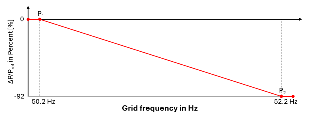
In this example at 50.2 Hz we are still allowed to feed 100% of the output power. If the frequency is rising against 52.2 Hz, we have to reduce to 92% of the nominal power. Other implementations can look like this, where the active power has a deadband of several deci-hertz while increasing the active power up to 200% at 47.5 Hz and reducing to 0% at 51.5 Hz linearily:
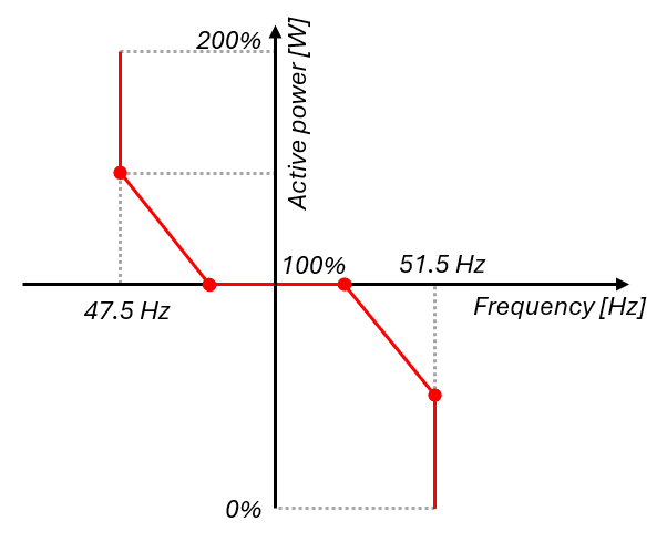
This allows a smooth control of the active power depending on the grid-frequency. Here a simple and slow integral-controller is sufficient. As more power increases the grid-voltage especially on weak grid-nodes, in addition to this P(f)-control the Q(U)-control comes into account. For instance, if a huge PV-power-plant is connected to a small grid-node with a long distance to the next grid-connection point, the impedance of this grid-node is much higher compared to a node that is closer to a grid substation. With higher grid-impedance the power fed into the grid will increase the voltage at this node. Without additional control the power of the PV-plant had to be decreased to keep the grid safe but we would loose the regenerative power. Here the reactive power can help to support the weak grid. An inductive reactive current creates a controlled voltage drop across the lines and transformers. This causes the excessively high grid voltage to drop back to a safe and normal level. Vice versa it is possible to support a weak grid with too low voltage by injecting capacitive reactive power so that the voltage rises back to its normal level:
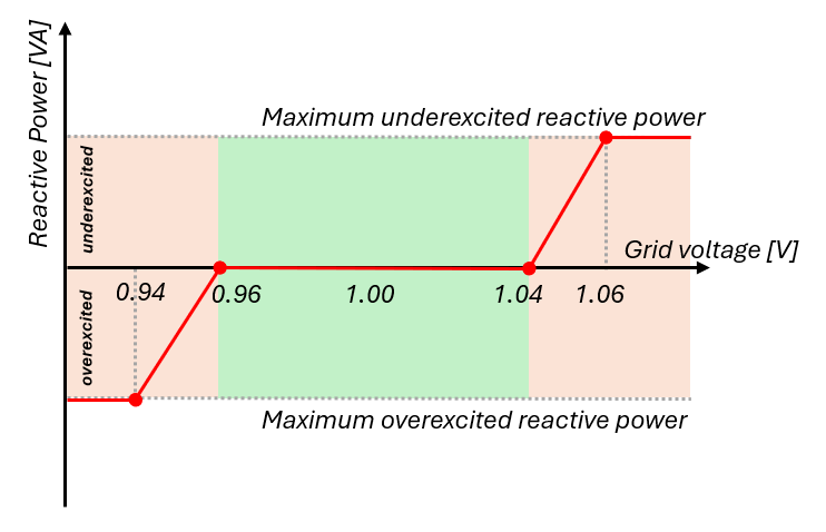
As we can control the active and reactive power independently with the d- and q-current, we have a very powerful set of tools using the vector-control.
Simulation
One of the benefits of modern simulation-tools is the integration. With PLECS we have the option to simulation either offline using the computer or online using the PLECS RT Box. First lets have a look at the simulation running as a regular simulation. The following curves show the initial connection to the grid after the PLL has locked. The curves at the top show the grid-voltages while the second curve shows the three grid-currents. The curve in the middle is displaying the input-current of the PV-modules followed by the DC-link-voltage in red and the input-voltage in green. The last curve shows the active power in green, the reactive power in red and the apparent power of the phase L1:
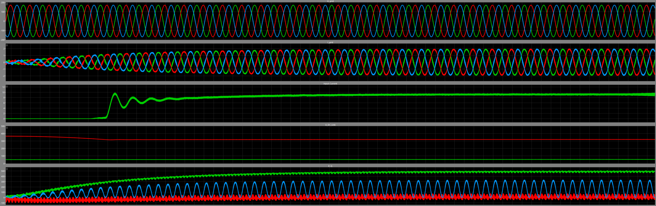
As we have “digital” switches here, the grid-current shows some disturbances caused by the turn-on and turn-off of the semiconductors. Here a better designed LCL-filter could reduce the harmonics even more:
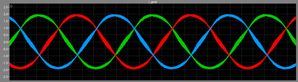
But in general the system is working. Now lets have a look at the P(f) and Q(U) controls. For this lets move to the online-simulation on the RT Box itsel. I will demonstrate the effects of both controls with two short videos. First lets have a look at the P(f) control. Lets start with a grid frequency of 50 Hz and reduce it down to 48 Hz. Right after this I will increase back to 50 Hz and then up to 52 Hz. Have a look at the active power in the last display: it will move between 500W (regular operation), 1000W (maximum output power) and 0W at maximum frequency:
The power-controller does its job and controls the maximum allowed power to the grid depending on the frequency. Now let’s switch to the reactive power part. Here the grid-voltage has to change to stimulate the second controller. In the following video I will change the grid-voltage from 120V down to 96V, then back to 120V and then up to 144V. Keep a spot on the red curve in the last diagram as well as the phase-shift of the grid-current with respect to the grid-voltage:
As both controls are working independently of each other both the grid-frequency and the grid-voltage will be compensated automatically.
More functions and conclusion
In summary, inverters are now able to interact with the grid and support it with the shown tools. Next to the P(f)- and Q(U)-control current inverters may support more features like the so called Fault-Ride-Through-capability. Here inverters will not disconnect during a short-circuit-like-event where the voltage collapses but will feed-in more power to support the grid until either the grid voltage gets back to a minimum value within 150ms or the inverter may disconnect from the faulty grid.
Another important thing is the ability to support blackstarting. Here the inverters can switch from grid-tied-mode to a grid-building mode and switch from current-controller to voltage-controller to act as a grid-building device. In this mode the inverter will create a small island-grid which then will synchronize and reconnect to another grid once it is available again.
In the case the inverter has access to a battery, the inverter could be connected via internet to build a so called virtual-power-plant. These systems can interact with each other or be controlled by a higher-level control system to optimize the battery-usage in combination of weather-forcasts, user-demands or EV-charging-events. So a lot of different things are possible now.
As you may have realized, I’m an absolute fan of sinewaves and inverters. I hope I’ve managed to get you a little excited about it with this blog post, too 🙂