
In my last post I showed how I used a neural network for a latency-free De-Feedback audio-plugin for live-applications. But as an electrical engineer for power electronics I was curious about how to use neural networks in control-algorithms.
Table of Contents
- Why using neural networks in control-loops?
- Creating training-data for the neural network
- Train the neural network
- Implementing neural network within the DLL in C-Code for PLECS
- Test of the new control
Why using neural networks in control-loops?
Most of the time a simple proportional- and integral-control (PI-controller) is enough for most of the basic applications. But sometimes there is a non-linear load or a specific application that requires a more enhanced control-loop. One example could be a grid-connected inverter where the grid introduces a 100Hz (for single-phase) or a 150Hz (for three-phase) disturbance in the DC-link. So the voltage- or current-controller has to deal with this disturbance. Sure, for this simple application we can use a feedback of this well-determinable disturbance with 180° to compensate the root of the problem, but sometimes this is not possible if the disturbance changes the frequency or is load-dependent.
To check the possible advantage of a neural-network I wanted to train a simple network and test it together with a simple buck-converter within the simulation-software PLECS:
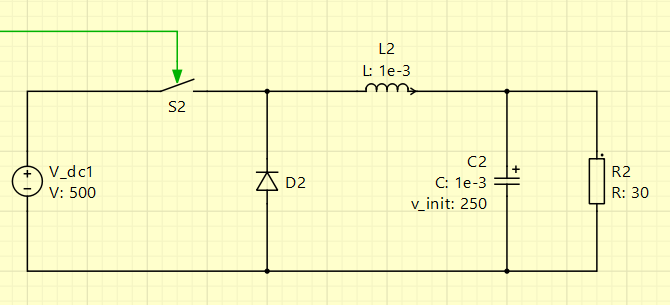
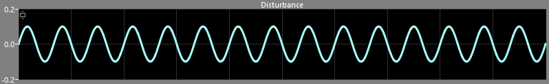
I’ve chosen a quite large capacitor of 1mF and modulated the dutycycle of 50% of the buck-converter with the following sine-wave, resulting in a dutycycle between 40% and 60%:
Combined with the large output-capacitor this produces quite high current-spikes as the capacitor is recharged wihtout damping when the switch is closed. As a result this produces a higher ripple in the output-voltage which is not welcome in a DC-to-DC-converter at all:
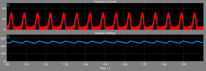
If we would stay with a common PI-control, we could increase the gain of the proportional- and integral-part and maybe add some derivative-parts, but the result is still not optimal:
Creating training-data for the neural network
The simulation-software PLECS has native support to use external DLL-files to run C-code directly. So I pondered how to integrate my neural network I used with the De-Feedback-plugin from last time. I also wondered how I could generate training data. My idea was to create two versions of the identical converter: one buck-converter with a simple PI-control with lower gain-values and another buck-converter with a 180°-feedback of the disturbance to compensate it entirely. This had the advantage, that I got the voltage-error of the bad-performing converter as well as the ideal-compensated converter.
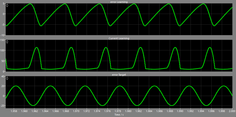
The following graph shows the voltage-error-signal of the converter with the standard PI-control at the top, the inductor-current in the center and the targeted voltage-error of the ideal-compensated converter at the bottom. These output-signals are sampled at switching-frequency – here 16kHz, which means a new sample every 62.5 microseconds:
As PLECS has the option to export the data of the scopes into a CSV-file I had a pretty easy way to export my training-data to individual files. Even better: the whole software can be automated using simulation-scripts as the software has GNU Octave as a backbone. Here is my script I used to export training-data for multiple different disturbances:
plecs('scope', './export', 'ClearTraces');
plecs('set', './AI_Control_EN', 'Value', '0');

amplitudeValues = [0.03, 0.1];
frequencyValues = [80, 100, 150];

for i = 1:length(amplitudeValues)
  for j = 1:length(frequencyValues)
    plecs('set', './Disturbance', 'Amplitude', mat2str(amplitudeValues(i)));
    plecs('set', './Disturbance', 'Frequency', ['2*pi*' mat2str(frequencyValues(j))]);

    plecs('simulate');

    plecs('scope', './export', 'ExportCSV', ['training_' mat2str(frequencyValues(j)) 'Hz_' mat2str(amplitudeValues(i)) '.csv'], [1 2]);
  end
end

plecs('set', './AI_Control_EN', 'Value', '1');The first lines clear any present values in the scope, disable the neural network control and prepare some vectors with some amplitude- and frequency-values for the artificial disturbance of the converter. Within the nested loop these values are set as parameters of the sine-wave-block in the simulation and the simulation is started. After each simulation-instance the data of the scope between second 1 and 2 is exported to a CSV-file. This ensures that the simulation has reached the steady-state and all lengths of the training-data are identical.
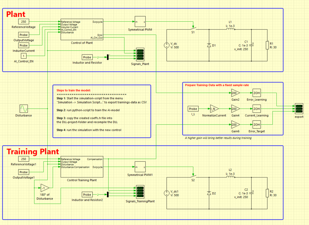
Here is the top-sheet of my simulation. The buck-converter with the uncompensated disturbance is at the top, while the ideal-compensated converter that is used as the target for the neural network is at the bottom. In the center you can see three signals that are connected to the export-scope already shown in the graph above:
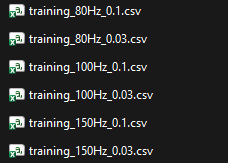
In the end I got 6 files with the voltage-error and the inductor-current as well as the desired voltage-error of the ideal-compensated control – each file with around only 1 megabyte:
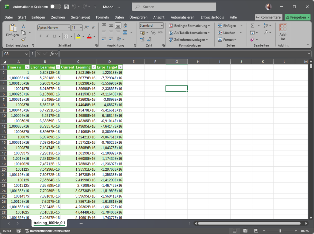
To get an idea of the data, here is a single file opened in Excel – just plain data-points over the time:
As you can see in the above graph of the three signals, the targeted voltage-error is not a perfect DC-signal, but just the compensation-part the neural network should output to compensate the disturbance. This means the trained neural network won’t be able to reach stationary accuracy so that we will use a slower integral-control in parallel to the neural network.
Train the neural network
As you might have realized, I’ve exported the inductor-current next to the voltage-error as an additional signal. It would be possible to train the network with just the voltage-error, but neural networks have the incredible advantage that they can handle multiple inputs. Just as a living being can use its eyes or senses like smelling or touching to detect heat for instance, a neural network can also use multiple inputs for control. As the sharp rise of the inductor-current is the cause for the voltage-ripple, we should be able to train the network to keep an “eye” exactly on this specific signal – next to the voltage-error of course.
But first I’d like to show you the changes I’ve done to the Python-script to train the neural network, compared to the last blog-post. In the previous post I used a non-linear filter combined with a gate that muted the channel if a feedback is detected. It was important to get a strong decision, if a feedback took place. That was the reason I’ve chosen the criterion “BCE With Logits Loss” that performs well on strong decisions. Now we need a continuous control-algorithm that compensates signals – so I’ve chosen the criterion “MSE Loss” that is beneficial on predicting continuous values:
def train_model_multi(trainingFiles, epoch_number=50, input_number=1, block_size=64, hidden_size=32):
    model = AiControlNet(input_size=block_size * input_number, hidden_size=hidden_size)
    criterion = nn.MSELoss()
optimizer = optim.Adam(model.parameters(), lr=0.001, weight_decay=1e-4)The learning-rate and other parameters are used like suggested in the PyTorch documentation. Even the batch-size and other parameters like the number of neurons in the hidden-layer are the same number as in the De-Feedback-plugin as I wanted to get a good starting point. The main difference is, that I created two different training-scripts: the first with only the voltage-error and the second with voltage-error and inductor-current. For this I simply doubled the input-size from 64 to 128. As I just wanted to see the general mechanism the number of multiplications were not important for me at this point. So here are the main-components of the training-script for the two-input-version:
import torch
import torch.nn as nn
import torch.optim as optim
import numpy as np
import pandas as pd
import os
import glob
class AiControlNet(nn.Module):
def __init__(self, input_size=64, hidden_size=32):
super(AiControlNet, self).__init__()
self.fc1 = nn.Linear(input_size, hidden_size)
self.tanh = nn.Tanh()
self.fc2 = nn.Linear(hidden_size, 1)
def forward(self, x):
x = self.fc1(x)
x = self.tanh(x)
x = self.fc2(x)
return x
def prepare_multi_data_csv(trainingFiles, block_size=64):
all_x = []
all_y = []
for input_csv in trainingFiles:
df_traningdata = pd.read_csv(input_csv)
# input data from CSV-file
input_error_learning = torch.tensor(df_traningdata["Error_Learning"].values, dtype=torch.float32)
input_current_learning = torch.tensor(df_traningdata["Current_Learning"].values, dtype=torch.float32)
input_error_target = torch.tensor(df_traningdata["Error_Target"].values, dtype=torch.float32)
min_len = len(input_error_target)
for i in range(min_len - block_size):
window_err = input_error_learning[i : i + block_size]
window_cur = input_current_learning[i : i + block_size]
combined_window = torch.cat([window_err, window_cur], dim=0)
all_x.append(combined_window.view(1, -1))
all_y.append(input_error_target[i + block_size - 1].view(1, 1))
x = torch.cat(all_x, dim=0)
y = torch.cat(all_y, dim=0)
indices = torch.randperm(x.size(0))
return x[indices], y[indices]
def train_model_multi(trainingFiles, epoch_number=50, input_number=1, block_size=64, hidden_size=32):
    model = AiControlNet(input_size=block_size * input_number, hidden_size=hidden_size)
    criterion = nn.MSELoss()
    optimizer = optim.Adam(model.parameters(), lr=0.001, weight_decay=1e-4)
inputs, labels = prepare_multi_data_csv(trainingFiles, block_size=block_size)
batch_size = 64
num_batches = len(inputs) // batch_size
for epoch in range(epoch_number):
epoch_loss = 0
perm = torch.randperm(len(inputs))
inputs = inputs[perm]
labels = labels[perm]
for i in range(num_batches):
start = i * batch_size
end = start + batch_size
batch_x = inputs[start:end]
batch_y = labels[start:end]
optimizer.zero_grad()
outputs = model(batch_x)
loss = criterion(outputs, batch_y)
loss.backward()
optimizer.step()
epoch_loss += loss.item()
if (epoch + 1) % 10 == 0:
print(f"Epoch {epoch+1}, Loss (MSE): {epoch_loss/num_batches:.6f}")
return modelTo call these two functions, I used the following code:
# get all CSV-files starting with "training" from the current folder
script_dir = os.path.dirname(os.path.abspath(__file__))
files = sorted(glob.glob(os.path.join(script_dir, "training_*.csv")))

if len(files) == 0:
    print("Error: no training-data found!")
    return

# setup the training
epoch_number = 100 # between 50 and 150 seems to be fine for basic buck-converter
input_number = 2 # voltage-error and current
block_size = 64 # input size of the network
hidden_size = 32 # size of neural network neurons

# train the model
model = train_model_multi(files, epoch_number=epoch_number, input_number=input_number, block_size=block_size, hidden_size=hidden_size)As in the De-Feedback-Plugin the result is a set of coefficients that can be used in C-Code or other languages to run the neural network:
nn_weights_Input_to_Hidden = model.fc1.weight.data.numpy()
nn_bias_Hidden = model.fc1.bias.data.numpy()
nn_weights_Hidden_to_Output = model.fc2.weight.data.numpy().flatten()
nn_bias_Output = model.fc2.bias.data.numpy()[0]Again, I exported all coefficients into a single C-header-file:
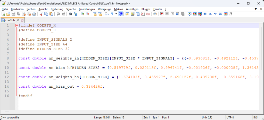
Implementing neural network within the DLL in C-Code for PLECS
Our goal is to calculate a compensation-signal that supports the work of the parallel PI-control lateron. So our control-algorithm has to take the voltage-error and the inductor-current, feed it into the neural network and return the compensation-signal back to the simulation. PLECS has a very nice DLL-interface so that it is very easy to interact with the simulation directly. Here is the full sourcecode of the C-DLL:
#include "main.h"

float get_nn_correction(float error, float current) {
    input_history[0][history_index] = error;
    input_history[1][history_index] = current;
    // increase index and wrap around if necessary
    int current_pos = history_index;
    history_index = (history_index + 1) % INPUT_SIZE;

    float hidden_layer[HIDDEN_SIZE];

    for (int i = 0; i < HIDDEN_SIZE; i++) {
        float sum = nn_bias_h[i];

		    // part 1: error-signal
        for (int j = 0; j < INPUT_SIZE; j++) {
            int idx = (history_index + j) % INPUT_SIZE;
            sum += nn_weights_ih[i][j] * input_history[0][idx];
        }

    		// part 2: current-signal
        for (int j = 0; j < INPUT_SIZE; j++) {
            int idx = (history_index + j) % INPUT_SIZE;
            sum += nn_weights_ih[i][j + INPUT_SIZE] * input_history[1][idx];
        }

    		hidden_layer[i] = tanhf(sum);
    }

    float delta_d = nn_bias_out;
    for (int i = 0; i < HIDDEN_SIZE; i++) {
        delta_d += nn_weights_ho[i] * hidden_layer[i];
    }

    return delta_d;
}

/*******************************
 FUNCTIONS FOR PLECS
********************************/

DLLEXPORT void plecsSetSizes(struct SimulationSizes* aSizes) {
	aSizes->numInputs = 2;
	aSizes->numOutputs = 1;
	aSizes->numStates = 0;
	aSizes->numParameters = 0;
}

DLLEXPORT void plecsStart(struct SimulationState* aState) {
	// aState->userData = malloc(sizeof(double) * 10);

	aState->errorMessage = NULL;
}

DLLEXPORT void plecsOutput(struct SimulationState* aState) {
	aState->outputs[0] = get_nn_correction(aState->inputs[0], aState->inputs[1]);
}

DLLEXPORT void plecsTerminate(struct SimulationState* aState) {
}If you compare the code of the function get_nn_correction() with the function nn_inference_scalar() from the De-Feedback-plugin, you can see that there are only minor changes:
- the history is moved to the beginning of the function
- the sum is calculated over the two inputs instead of only one input
- the hidden-layer is now calculated using the function tanhf() instead of a binary-function
- the output is not a sigmoid-function anymore but the weighted output of the hidden layer is used directly
To compile the DLL I’ve downloaded GCC for Windows and compiled the code with the following command:
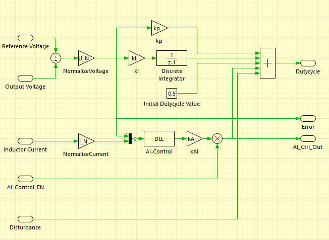
C:\gcc\bin\gcc.exe -shared -o NeuralNetworkControl.dll main.c -m64That’s it. Here is a picture of the sub-system “Control of Plant” shown in the image of the whole PLECS-simulation, that contains the proportional- and integral-controller, an initial dutycycle of 50% as well as the neural-network-DLL-block:
Test of the new control
OK, let’s get down to business. The DLL is compiled, the simulation is ready. Remember, this was the inductor-current and the output-voltage of the buck-converter without the neural network:
Pretty sharp current-spikes while fast-charging the capacitor, resulting in the shown voltage-ripple. And this is the result of my first version of the neural network with just the voltage-error as an input:

The peak of the inductor-current could be reduced from around 45 A down to 32 A, but the control struggles with the sharp current-slope. As the neural network has only knowledge about the voltage-error as a result of the high charging-current of the inductor, our network can only react to the outcome of the current. But things change dramatically for the better when we feed significantly more information into the neural network by using the inductor current:
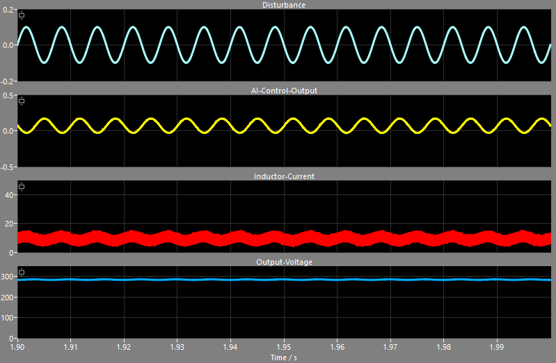
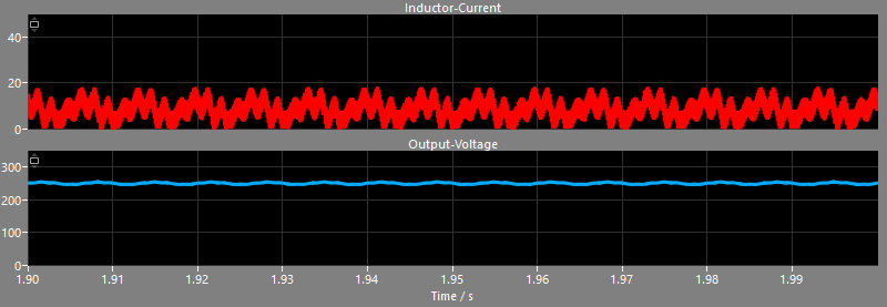
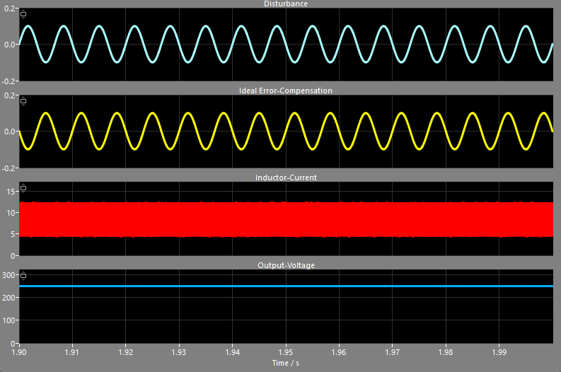
This is the result of just the neural network without the PI-control. The voltage is too high – around 280V instead of the desired 250V, but the network is able to reduce the peak-currents down to a nice 10A +/- 5A. Using a slow PI-controller in parallel to the neural network controller solves the problem with the voltage-offset and the buck-converter shows a much cleaner output-voltage at 250V:
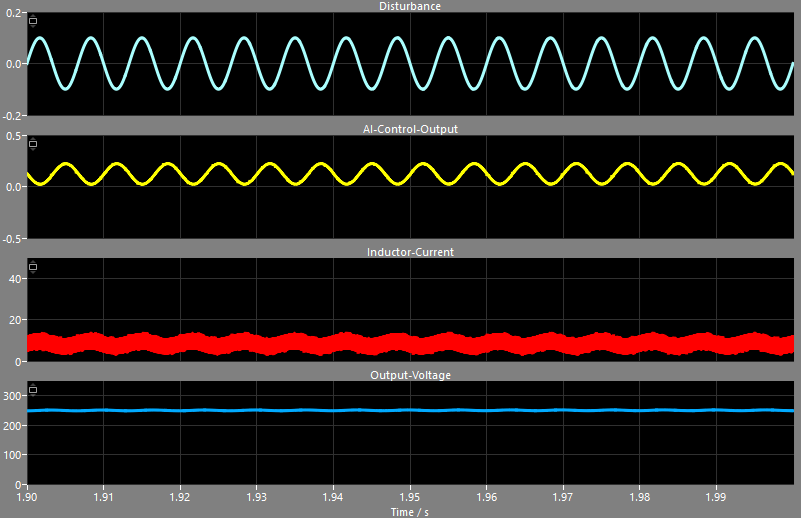
For comparison, these are the signals using the ideal compensation of the artificial disturbance:
So with 32 neurons in the hidden-layer the neural network is able to detect the specific disturbance, is aware of the relation between inductor current and output-voltage and can output a proper dutycycle-correction. Sure, this controller needs much more multiplications and memory compared to a simple PI-controller, but if the performance of a converter with a difficult load can be improved drastically, it could be worth the efford – and microcontrollers are getting cheaper and cheaper.